Authors
- Brin Rosenthal, Ph.D. (sbrosenthal@ucsd.edu)
- Julia Len (jlen@ucsd.edu)
- Mikayla Webster (m1webste@ucsd.edu)
- Aaron Gary (agary@ucsd.edu)
- Kathleen Fisch, Ph.D (kfisch@ucsd.edu)
License
This project is licensed under the MIT License - see the LICENSE file for details
visJS2jupyter is a tool to bring the interactivity of networks created with vis.js into jupyter notebook cells, authored by members of the UCSD Center for Computational Biology & Bioinformatics
Table of contents
- Getting started
- Features and examples
- Supplemental Information
3.1. Tips on usage
3.1.1 Multiple networks in the same notebook
3.1.2 Mapping colors to nodes and edges
3.1.3 High resolution images
3.1.4 Exporting to Cytoscape compatible format
3.2. Visualizations
3.2.1 Graph Overlap
3.2.2 Heat propagation
3.2.3 Co-localization
3.3. Validating network propagation with known Autism risk genes
3.4. Arguments
3.4.1 Required arguments
3.4.2 Node-specific arguments
3.4.3 Edge-specific arguments
3.4.4 Interaction-specific arguments
3.4.5 Configuration-specific arguments
3.4.6 Miscellaneous arguments
Getting started
These instructions will get you a copy of the package up and running on your local machine.
Prerequisites
You must have Jupyter notebook already installed. Visit here for more information.
Install matplotlib before using visJS2jupyter. Visit here for more information.
To use the visualizations module, install networkX and py2cytoscape:
pip install networkx
pip install py2cytoscape
Installing
visJS2jupyter supports both Python 2.7 and 3.4.
You can install visJS2jupyter using pip:
pip install visJS2jupyter
In your Jupyter notebook, first import matplotlib:
import matplotlib
To import visJS_module, use the following:
import visJS2jupyter.visJS_module
To import visualizations, use the following:
import visJS2jupyter.visualizations
Features and examples
Simple example: A simple use example with default parameters may be found here. In the example provided, we show how to display a graph created with NetworkX using visJS2jupyter. The networks displayed within Jupyter notebook cells may be dragged, clicked, and hovered on, and zooming is enabled within the window.
More complex example:For an example of how more complex styles may be added to a network, see this example. Nodes and edges may be styled with properties available from vis.js networks (see http://visjs.org/docs/network/ for a list and description of properties). The main function is ‘visjs_network’, which requires two inputs which describe the nodes and edges in the network- ‘nodes_dict’, and edges_dict’. The other arguments are optional, and apply general styles to the graph, such as sizes, highlight colors, and physics properties of the graph.
Load MI-TAB network:An example showing how to load network data in MI-TAB format is found here. In this example, reactome data in MI-TAB format is loaded, mapped to a networkX network, with corresponding edge attributes pulled from the MI-TAB table, and uniprot IDs are mapped to HGNC gene symbols using the MyGene.info python tool. The largest connected component of this graph is visualized with visJS2jupyter, with edge colors corresponding to interaction type, and node sizes indicating degree (number of connections).
TCGA common mutations:An biologically inspired interactive use example of visJS2jupyter may be found here (scroll to the bottom to see the network). In this example, we display the bipartite network composed of diseases in The Cancer Genome Atlas and the top 25 most common mutations in each disease. We also overlay information about drugs which target those mutations. Genes which have a drug targeting them are displayed with a bold black outline. The user may hover over each gene to get a list of associated drugs.
Prioritize autism risk genes:An example of how to use the network propagation functionality of our tool to prioritize genes related to autism is located here
Multigraph example:For an example of how to style a multigraph using visJS2jupyter, see https://bl.ocks.org/m1webste/raw/db4aeda3f3e4a8840f08182f2e5d4608/ This notebook demonstrates how to use visJS2jupyter to visualize a NetworkX multigraph inside a jupyter notebook cell. visJS2jupyter can be used to manipulate numerous graph styling parameters (edge width, node color, node spacing, etc.). In this notebook, we exemplify manipulating a small subset of these features. Notibly, we demonstrate how to manipulate node and edge colors for a multigraph based off of node and edge attributes.
Visualizations
Supplementary module, containing frequently used network visualizations
1) draw_graph_overlap takes in two graphs and displays their overlap. Intersecting nodes are triangles and non-intersecting nodes are either circles or squares, depending on which graph they belong to. An interactive example may be found here. In this example, we graph the union of two networks of 10 nodes each. The user can hover over each node to see the graph it belongs to and the node name.
2) draw_heat_prop simulates heat propagation on the network initialized from a given set of seed nodes. It takes in a graph and a list of seed nodes. An interactive example may be found here.
3) draw_colocalization similarly draws the heat propagation of the graph but with two sets of seed nodes. Another interactive example can be found here.
Supplemental Information
3.1 Tips on usage
3.1.1 Multiple networks in the same notebook
visJS2jupyter takes parameters specified by the user and then creates an HTML file that contains the vis.js code to draw the network visualization. Each graph generates its own HTML file. The Jupyter notebook cell then renders this HTML file to produce the visualization. To create multiple graphs in one notebook, use the graph_id argument to specify an identification for the graph. Each different graph_id will generate a different HTML file.
3.1.2 Mapping colors to nodes and edges
Color-coding nodes and edges is a common way of mapping complex layers of information to a graph. The functions return_node_to_color and return_edge_to_color included in the package provide the means with which to do this. The return_node_to_color function creates a dictionary mapping of nodes to color values based on the specified colormap and node attribute to map. Similarly, return_edge_to_color creates a dictionary mapping of edges to color values. Any node or edge level property can be mapped to node color or edge color, as long as it is represented numerically, and added as a node/edge attribute. Use the argument field_to_map to specify this property. The user can also utilize the argument cmap to specify which matplotlib colormap to use for the color mapping.
3.1.3 High resolution images
In order to save high resolution images, we include the ‘scaling_factor’ argument, which scales up each graph element and increase its resolution. To save the image, right-click on the notebook cell and select ‘save as’. For most graphs an adequately high-resolution image is obtained from setting the scaling_factor between three and five.
3.1.4 Exporting to cytoscape compatible format
To export to a cytoscape compatible format, set the ‘export_network’ argument to True in the visualization functions. The network, with attributes, will be saved in a Cytoscape compatible JSON format. To change the default file name, set the ‘export_file’ argument to the desired name. Once the network has been saved, open Cytoscape and load the file. To reproduce the network as it looked in the Jupyter cell, load the corresponding Cytoscape style file (provided where in the GitHub repository https://github.com/ucsd-ccbb/visJS2jupyter/tree/master/cytoscape_styles), and apply it to the network.
Note that physics simulations will interfere with the initial placement of nodes and edges in the network. Thus, to reproduce the network exactly, we recommend keeping the physics simulation turned off.
3.2. Visualizations
Visualizations is a supplementary module that calls visJS_module to perform operations on graphs, and to visualize their results. These functions include the overlap of two graphs, heat propagation, and co-localization. Users simply provide a network in NetworkX format, and when called, the function performs the desired operation. The function then visualizes the output in the notebook cell. Many customizations are possible for the graph, such as the color maps used for nodes and edges. Furthermore, users can customize the physics simulation of their networks. The physics simulation provides another interactive element of the graph that enables users to view the connectivity of nodes when dragging them. By default, the physics simulation is turned on for networks of fewer than 100 nodes and turned off otherwise. All arguments available in visJS_module for network customization are also available in visualizations.
3.2.1 Graph overlap
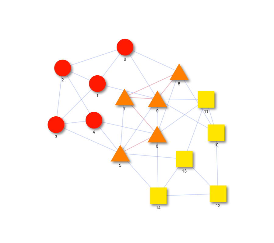
When working with networks, it is often useful to consider how similar two networks are. The function draw_graph_overlap introduces a network overlap visualization function to allow comparisons between networks. This function takes in two NetworkX graphs and displays a single graph of their union. Intersecting nodes are triangles and non-intersecting nodes are either circles or squares, depending on which graph they belong to. A simple example can be found at https://bl.ocks.org/julialen/raw/d21c9d378cb09b5a7181497101996727/.
Figure S2: Graph of the overlap between two networks using draw_graph_overlap. Nodes in the intersection of the networks are orange triangles, while edges in the intersection are colored red.
3.2.2 Heat propagation
We implement the network propagation method developed in (Vanunu et al. 2010), which simulates how heat would diffuse, with loss, through the network by traversing the edges, starting from an initially hot set of ‘seed’ nodes. At each step, one unit of heat is added to the seed nodes, and is then spread to the neighbor nodes. A constant fraction of heat is then removed from each node, so that heat is conserved in the system. After a number of iterations, the heat on the nodes converges to a stable value. This final heat vector is a proxy for how close each node is to the seed set. For example, if a node was between two initially hot nodes, it would have an extremely high final heat value, and alternatively if a node was quite far from the initially hot seed nodes, it would have a very low final heat value. This process is described in (Vanunu et al. 2010):
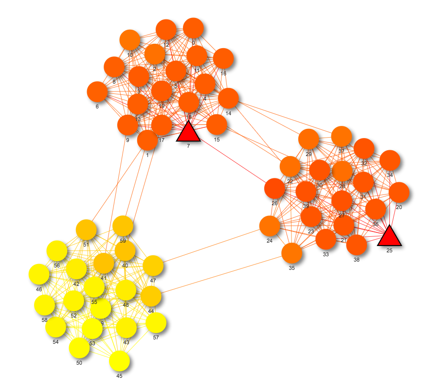
Heat propagation is useful for visualizing network propagation from a set of seed nodes. The function draw_heat_prop draws this visualization when provided with a NetworkX graph and a list of seed nodes. Using the list of seed nodes, it calculates the heat value of each node based on how connected it is to the seed nodes. Seed nodes are depicted with a triangular shape to distinguish them from other nodes. By default, hot nodes are colored red with cooler nodes gradually fading to yellow. The edges are also colored from red to yellow, depending on the heat of the nodes they are connecting. The overall effect is a clear visualization of how the heat from the seed nodes spreads throughout the network. If including all nodes in the graph produces a cluttered network, draw_heat_prop provides the argument ‘num_nodes’ to specify how many nodes the network should include. This argument finds the num_nodes number of hottest nodes and only graphs those. An example of a network drawn by draw_heat_prop can be found at https://bl.ocks.org/julialen/raw/82c316048ade650effbff3fd9eaddccd/.
Figure S3: Network propagation of a three-cluster network with two seed nodes using draw_heat_prop. Seed nodes are red triangles.
3.2.3 Co-localization
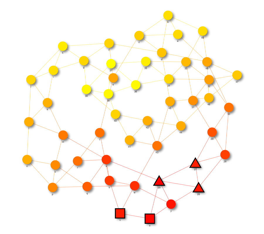
Co-localization works similarly to heat propagation but requires two sets of seed nodes instead of one. The function draw_colocalization creates a network visualization of this propagation. Seed nodes belonging to one set are shaped as triangles while seed nodes belonging to the other set are shaped as squares. Heat values are calculated by running a heat propagation simulation with one set of seed nodes and then a different propagation using the other set of seed nodes. The product of the heat values in each simulation becomes each node’s heat value in the final graph. An example can be found at https://bl.ocks.org/julialen/raw/a82040bdc8b5ba3ca866489db795af74/.
Figure S4: Co-localization of network from two sets of seed nodes using draw_colocalization. Seed nodes from one set are red squares, while seed nodes from the other set are red triangles.
3.3. Validating network propagation with known Autism risk genes
We validate the network propagation technique as a method for prioritizing disease risk genes, from a set of genes known to be involved in the disease. We start with the large set of genes known to be involved in Autism, as our set of seed genes, and the STRING (REF) interactome as our background network for propagation.
To test if the network propagation function will be useful for gene prioritization, we randomly select a subset of n genes from the total list of 859, run the network propagation function from these n genes on the STRING interactome, and then count the number of withheld Autism genes which appear in the top N hottest genes. If the method works, we will find many withheld Autism genes in the top set, because we expect disease-related genes to be near other disease-related genes, in network space. To establish a baseline, we run a control condition. We randomly select 859 control genes, C from the genome, and repeat the prioritization test on this set. That is, we randomly select n genes from the control set C to use as seeds for the network propagation, and measure the number of withheld control genes which are recovered in the top N hottest genes. This experiment is repeated k=100 times for each value of N (Figure ??, where we plot the fraction of recovered withheld disease risk genes recovered for Autism (red) and Control (black)). Consistently we recover many more Autism genes than Control genes, in the simulation, indicating that the network propagation method works as a prioritization technique, as expected.
Analysis for this result may be found in Jupyter notebook form (HERE).
3.4. Arguments
3.4.1 Required arguments
nodes_dict: A list of information about each node. Each node should have its own dictionary that must include ‘id’, the id of the node; ‘x’, the node x position; and ‘y’, the node y position. Other optional properties can be included to customize each individual node. The following is the current list of properties that can be modified at the node level:
- ‘border_width’
- ‘color’
- ‘degree’
- ‘node_label’: the label given to each node
- ‘node_shape’: The possible options are ‘ellipse’, ‘circle’, ‘database’, ‘box’, ‘text’, ‘image’, ‘circularImage’, ‘diamond’, ‘dot’, ‘star’, ‘triangle’, ‘triangleDown’, ‘square’, and ‘icon’.
- ‘node_size’
- ‘title’: the hover information of the node
- ‘x’: x-coordinate of the node within the graph
- ‘y’: y-coordinate of the node within the graph
edges_dict: A list of information about each edge. Each edge should have its own dictionary that must include ‘source’ and ‘target’, which refer to the integer ids of the source and target nodes. Other customizations for each edge can also be specified, such as ‘color’ and ‘title’.
Because of the way visJS2jupyter interprets node and edge data, before creating edges_dict, it is useful to create a node map that maps the names of nodes to integers. This can be done with the following line of code:
node_map = dict(zip(nodes, range(len(nodes))))
where nodes refers to the list of all nodes in the graph. Then, edges_dict can be created with the following:
edges_dict = [{“source”:node_map[edges[i][0],
             “target”:node_map[edges[i][1]}
             for i in range(len(edges))]
where edges refers to the list of all edges in the graph.
Note: Many of the following arguments are customized features that come directly from vis.js. To view a more comprehensive description for these arguments, the full documentation can be found at http://visjs.org/docs/network/.
3.4.2 Node-specific arguments
node_border_width: integer (default = 2)
Node border width when not hovered on or selected.
node_border_width_selected: integer (default = 2)
Node border width once clicked.
node_broken_image: string (default = ‘undefined’)
Name of backup image in case a node image doesn’t successfully load.
node_color_border: string (default = ‘black’)
Creates border around node shape in specified color.
node_color_highlight_border: string (default = ‘#2B7CE9’)
Node border color when selected.
node_color_highlight_background: string (default = ‘orange’)
Border color when selected.
node_color_hover_border: string (default = ‘#2B7CE9’)
Color of node border when mouse hovers but does not click.
node_color_hover_background: string (default = ‘orange’)
Color of node when mouse hovers but does not click.
node_fixed_x: boolean (default = False)
Node does not move in x direction but is still calculated into physics.
node_fixed_y: boolean (default = False)
Node does not move in y direction but is still calculated into physics.
node_font_color: string (default = ‘#343434’)
Color of label text.
node_font_size: integer (default = 14)
Size of label text.
node_font_face: string (default = ‘arial’)
Font face of label text.
node_font_background: string (default = “rgba(0,0,0,0)”)
When defined with color string, a background rectangle will be drawn around text.
node_font_stroke_width: integer (default = 0)
Width of stroke. If zero, no stroke is drawn.
node_font_stroke_color: string (default = ‘#ffffff’)
Color of stroke.
node_font_align: string (default = ‘center’)
Alignment of node font. Other option is ‘left’.
node_icon_face: string (default = ‘FontAwesome’)
Only used when shape is set to icon. Options are ‘FontAwesome’ and ‘Ionicons’.
node_icon_code: string (default = ‘undefined’)
Code used to define which icon to use.
node_icon_size: integer (default = 50)
Size of icon.
node_icon_color: string (default = ‘#2B7CE9’)
Color of icon.
node_image: string (default = ‘undefined’)
When shape set to ‘image’ or ‘circularImage’, then the URL image designated here will be used.
node_label_highlight_bold: boolean (default = True)
Determines if label emboldens when node is selected.
node_scaling_min: integer (default = 10)
Minimum size node can become when it scales down.
node_scaling_max: integer (default = 30)
Maximum size node can become when it scales up.
node_scaling_label_enabled: boolean (default = False)
Toggle scaling of label on or off.
node_scaling_label_min: integer (default = 14)
Minimum font size the label can become when it scales down.
node_scaling_label_max: integer (default = 30)
Maximum font size the label can become when it scales up.
node_scaling_label_max_visible: integer (default = 30)
Font will never be larger than this number at 100% zoom.
node_scaling_label_draw_threshold: integer (default = 5)
The lower limit of what the font is drawn as. Use this and node_scaling_label_max_visible to control which labels remain visible during zoom out.
node_shadow_enabled: boolean (default = True)
Whether there is a shadow cast by the nodes.
node_shadow_color: string (default = ‘rgba(0,0,0,0.5)’)
Shadow color.
node_shadow_size: integer (default = 10)
Shadow blur size.
node_shadow_x: integer (default = 5)
Shadow x offset from node.
node_shadow_y: integer (default = 5)
Shadow y offset from node.
node_shape_border_dashes: boolean (default = False)
Makes dashed border around node.
node_shape_border_radius: integer (default = 6)
Determines roundness of node shape (only for “box” shape).
node_shape_interpolation: boolean (default = True)
Only for image and circular image. Image resamples when scaling down.
node_shape_use_image_size: boolean (default = False)
Only for image and circular image. True means use image size, and False means use the defined node size.
node_shape_use_border_with_image: boolean (default = False)
Only for image. Draws border around image icon.
node_label_field: string (default = ‘id’)
Field that nodes will be labeled with.
node_size_field: string (default = ‘degree’)
Field that determines which nodes are more important and thus should be scaled bigger.
node_size_transform: string (default = ‘Math.sqrt’)
Function by which higher value (not node_value) nodes are scaled larger to show importance.
node_size_multiplier: integer (default = 3)
Increment by which higher value (not node_value) nodes are scaled larger to show importance.
3.4.3 Edge-specific arguments
edge_title_field: string (default = ‘id’)
The name of the attribute to show on edge hover.
edge_arrow_to: boolean (default = False)
Creates a directed edge with arrow head on receiving node.
edge_arrow_from: boolean (default = False)
Creates a directed edge with the arrow head coming from the delivering node.
edge_arrow_middle: boolean (default = False)
Creates a directed edge where arrow is in center of edge.
edge_arrow_to_scale_factor: integer (default = 1)
Changes size of “to” arrow head.
edge_arrow_from_scale_factor: integer (default = 1)
Changes size of “from” arrow head.
edge_arrow_middle_scale_factor: integer (default = 1)
Changes size of middle arrow head.
edge_arrow_strikethrough: boolean (default = True)
When False, edge stops at arrow.
edge_color: string (default = ‘#848484’)
If all edges are to be a single color, specify here. Empty string refers edge color to each individual object.
edge_color_highlight: string (default = ‘#848484’)
If all edge highlights are to be a single color, specify here. Empty string refers edge color highlight to each individual object.
edge_color_hover: string (default = ‘#848484’)
If all edge hover color are to be a single color, specify here. Empty string refers edge hover color to each individual object.
edge_color_inherit: string (default = ‘from’)
If edge color is set, must be false. Otherwise, inherits color from “to”, “from”, or “both” connected node.
edge_color_opacity: float (default = 1.0)
Number from 0 - 1 that sets opacity of all edge colors.
edge_dashes: boolean (default = False)
If true, edges will be drawn with a dashed line.
edge_font_color: string (default = ‘#343434’)
Color of label text.
edge_font_size: integer (default = 20)
Size of label text.
edge_font_face: string (default = ‘arial’)
Font of label text.
edge_font_background: string (default = ‘rgba(0,0,0,0)’)
When given a color string, a background rectangle of that color will be drawn behind the label.
edge_font_strokeWidth: integer (default = 0)
Width of stroke drawn around text.
edge_font_stroke_color: string (default = ‘#343434’)
Color of stroke.
edge_font_align: string (default = ‘horizontal’)
Alignment of font. Options are ‘horizontal’, ‘middle’, ‘top’, or ‘bottom’.
edge_hoverWidth: float (default = 0.5)
The value to be added to the edge width when the user hovers over the edge with the mouse.
edge_label_highlight_bold: boolean (default = True)
Determines whether label becomes bold when edge is selected.
edge_length: string (default = ‘undefined’)
When a number is defined, the edges’ spring length is overridden.
edge_scaling_min: integer (default = 1)
Minimum allowed edge width value.
edge_scaling_max: integer (default = 15)
Maximum allowed edge width value.
edge_scaling_label_enabled: boolean (default = False)
When true, the label will scale with the edge width.
edge_scaling_label_min: integer (default = 14)
Minimum font size used for labels when scaling.
edge_scaling_label_max: integer (default = 30)
Maximum font size used for labels when scaling.
edge_scaling_label_max_visible: integer (default = 30)
Maximum font size of label will zoom in.
edge_scaling_label_draw_threshold: integer (default = 5)
Minimum font size of label when zooming out.
edge_selection_width: integer (default = 1)
The value to be added to the edge width when the edge is selected.
edge_selfReferenceSize: integer (default = 10)
When there is a self-loop, this is the radius of that circle.
edge_shadow_enabled: boolean (default = False)
Whether or not a shadow is cast.
edge_shadow_color: string (default = ‘rgba(0,0,0,0.5)’)
Color of shadow as a string.
edge_shadow_size: integer (default = 10)
Blur size of shadow.
edge_shadow_x: integer (default = 5)
The x offset of the edge shadow.
edge_shadow_y: integer (default = 5)
The y offset of the edge shadow.
edge_smooth_enabled: boolean (default = False)
Toggle smoothed curves. If this is set to True and smooth type is not continuous, you will not be able to set the x and y position.
edge_smooth_type: string (default = ‘dynamic’)
The type of smooth curve drawn. Options include ‘dynamic’, ‘continuous’, ‘discrete’, ‘diagonalCross’, ‘straightCross’, ‘horizontal’, ‘vertical’, ‘curvedCCW’, and ‘cubicBezier’.
edge_smooth_force_direction: string (default = ‘none’)
Only for cubicBezier curves. Options are ‘horizontal’, ‘vertical’, and ‘none’.
edge_smooth_roundness: float (default = 0.5)
Number between 0 and 1 that changes roundness of curve, except with dynamic curves.
edge_width: integer (default = 1)
Width of all edges.
edge_label_field: string (default = ‘id’)
Field that edges will be labeled with.
edge_width_field: string (default = ‘’)
Field specifying edge width. If blank, defaults to global edge_width value for all edges. Otherwise, overrides the global value with the numeric value from that field.
3.4.4 Interaction-specific arguments
drag_nodes: boolean (default = True)
When True, the nodes that are not fixed can be dragged by the user.
drag_view: boolean (default = True)
When true, the view can be dragged around by the user.
hide_edges_on_drag: boolean (default = False)
When True, the edges are not drawn when dragging the view. This can greatly speed up responsiveness on dragging, improving user experience.
hide_nodes_on_drag: boolean (default = False)
When True, the nodes are not drawn when dragging the view. This can greatly speed up responsiveness on dragging, improving user experience.
hover: boolean (default = True)
When True, the nodes use their hover colors when the mouse moves over them.
hover_connected_edges: boolean (default = True)
When True, on hovering over a node, its connecting edges are highlighted.
keyboard_enabled: boolean (default = False)
Toggle the usage of the keyboard shortcuts. If this option is not defined but any of the other keyboard related options are, it is set to True.
keyboard_speed_x: integer (default = 10)
The speed at which the view moves in the x direction on pressing a key or pressing a navigation button.
keyboard_speed_y: integer (default = 10)
The speed at which the view moves in the y direction on pressing a key or pressing a navigation button.
keyboard_speed_zoom: float (default = 0.02)
The speed at which the view zooms in or out pressing a key or pressing a navigation button.
keyboard_bind_to_window: boolean (default = True)
When binding the keyboard shortcuts to the window, they will work regardless of which DOM object has the focus. If you have multiple networks on your page, you could set this to false, making sure the keyboard shortcuts only work on the network that has the focus.
multiselect: boolean (default = False)
When True, a longheld click (or touch) as well as a control-click will add to the selection.
navigation_buttons: boolean (default = False)
When True, navigation buttons are drawn on the network canvas. These are HTML buttons and can be completely customized using CSS.
selectable: boolean (default = True)
When True, the nodes and edges can be selected by the user.
select_connected_edges: boolean (default = True)
When True, on selecting a node, its connecting edges are highlighted.
tooltip_delay: integer (default = 300)
When nodes or edges have a defined ‘title’ field, this can be shown as a pop-up tooltip. The tooltip itself is an HTML element that can be fully styled using CSS. The delay is the amount of time in milliseconds it takes before the tooltip is shown.
zoom_view: boolean (default = True)
When True, the user can zoom in.
3.4.5 Configuration-specific arguments
config_enabled: boolean (default = False)
Toggle the configuration interface on or off. This is an optional parameter. If left undefined and any of the other configuration properties are defined, this will be set to True.
config_filter: string (default = ‘nodes,edges’)
When a string is supplied, any combination of the following is allowed: nodes, edges, layout, interaction, manipulation, physics, selection, renderer. Feel free to come up with a fun separating character. Finally, when supplied an array of strings, any of the previously mentioned fields are accepted.
container: string (default = ‘undefined’)
This allows you to put the configure list in another HTML container than below the network.
showButton: boolean (default = False)
Show the generate options button at the bottom of the configurator.
3.4.6 Miscellaneous arguments
border_color: string (default = ‘white’)
Border color of the network image element.
physics_enabled: boolean (default = True)
Toggle the physics system simulation on or off.
min_velocity: integer (default = 2)
Set the minimum velocity of nodes in the physics simulation. Once all nodes reach this velocity, the network is assumed to be stabilized and the simulation stops.
max_velocity: integer (default = 8)
Set the maximum velocity of nodes in the physics simulation.
draw_threshold: integer (default = None)
Deprecated argument: use node_scaling_label_draw_threshold and edge_scaling_label_draw_threshold. If used, node_scaling_label_draw_threshold and edge_scaling_label_draw_threshold are assigned the value of draw_threshold.
min_label_size: integer (default = None)
Deprecated argument: use node_scaling_label_min and edge_scaling_label_min. If used, node_scaling_label_min and edge_scaling_label_min are assigned the value of min_label_size.
max_label_size: integer (default = None)
Deprecated argument: use node_scaling_label_max and edge_scaling_label_max. If used, node_scaling_label_max and edge_scaling_label_max are assigned the value of max_label_size.
max_visible: integer (default = None)
Deprecated argument: use node_scaling_label_max_visible
and edge_scaling_label_max_visible. If used, node_scaling_label_max_visible and edge_scaling_label_max_visible are assigned the value of max_visible.
graph_title: string (default = ‘ ’)
Sets the title of the graph network.
graph_width: integer (default = 900)
Sets the width of the canvas.
graph_height: integer (default = 800)
Sets the height of the canvas.
scaling_factor: integer (default = 1)
To scale the image up, the graph network will scale up by the value provided. This argument is helpful when wanting to save a high resolution image of the network.
time_stamp: integer (default = 0)
Deprecated argument: use graph_id. If used, graph_id is assigned the value of time_stamp.
graph_id: integer (default = 0)
To draw multiple graphs in the same notebook, you must use this argument to give each graph a different id.
override_graph_size_to_max: boolean (default = False) If set to true, overrides the graph_width and graph_height pixel values to use 100% of available space. Useful for html and jupyter output, but not recommended for zeppelin. Do not use this with scaling_factor other than 1.
output: string (default = ‘jupyter’) When not set, produces output for jupyter to be used as usual. When set to “zeppelin”, you can simply print the returned value in the zeppelin notebook. When set to “html”, it will return the raw full HTML code which you can save to a file. When set to “div”, it will return a Python dictionary with separate code snippets you can embed into different sections of your custom HTML file.